Lane Following using Pure Pursuit Controller on F1TENTH Car
Welcome! This is our final project for course ECE484-Principles-Of-Safe-Autonomy in 2023 Fall. The course page can be found here.
The project implements a vision-based lane following system. Our aim to make vehicle follow the lane accurately and quickly without collision using Pure Pursuit Controller given RGB images. Our vehicle platform is build on F1TENTH.
Please check out our final presentation video for brief summary for the proejct.
1 - Overview
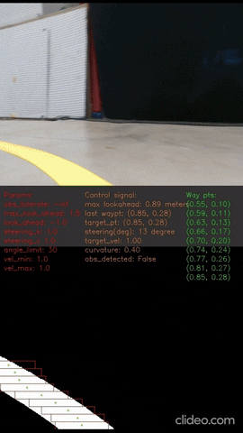
The vehicle is able to follow the lane accurately without collision:
2 - Method
The project built vision-based lane following system from scratch. Lane detector identifies the lane from the captured frame and provides candidates of imaginary waypoint for the controller. Next, the controller selects the best waypoint based on the vehicle state, and sends out next control signal.
The whole system is integrated with ROS, consisting of three primary components:
- Camera calibration
- Lane detection
- Controller
Component 1: Camera calibration
Inches to pixels
Because the target yellow lane must stick on the ground, we can simply measure the relationship between inches and pixels by applying the projection matrix $P_{measure}$ to a planar board lying on the ground.
View-widen trick
As Figure 2 shows, pixels of white board in camera view take up the entire area in measured bird-eye view. That is to say, the other pixels in camera view is invisible in measured bird-eye view.
An intuitive question pops up: What if different project matrix $P_{detection}$ is used in lane detection, e.g.$P_{detection} \neq P_{measure}$? Can we still derive the real-world inches of detected waypoints? (We will walk through lane detection later)
Yes, we can solve the problem through a combination of linear transformation as Figure 3 shows.
Component 2: Lane detection
demo:
Lane detection steps:
Perspective tranform Apply projection matrix $P_{detection}$ metioned in section “view-widen trick”.
Thresholding
- Hue thresholding: lane’s hue should lie between hue_min and hue_max.
Value thresholding: the blue channel value should exceed a specified threshold compared to the red channel value. Our choice of utilizing multiple channels instead of a grayscale value results from experiments.
Saturation thresholding: we found that saturation channel can well separate the histogram distribution between background and lane across most of the frames. All we have to do is find a dividing point somewhere between as Figure 5 shows. We use cumulative distribution function(CDF) to achieve this goal. Dividing point is defined as the bin with minimum pixel number between certain CDF ratio range as Figure 6 shows.
Figure 5: saturation histogram. Figure 6: saturation thresholding with CDF. Note that a heuristic is introduced is that the bin with minimum pixel number will appear between CDF 0.6 to 0.9. Lane fit Vertically adjust the window box progressively based on detected lane pixels. The initial center of the box, denoted as $w_{t}$, relies on the slope calculated from the centers of the previous two windows $w_{t-1}$ and $w_{t-2}$. Then we refine the center of each box by computing the mean of the x positions of the lane pixels included within the box. The process ends when $w_{t}$ reaches the image boundary or the number of detected pixels drops below a certain threshold.
Component 3: Controller
Longitudinal controller
We apply the dynamic speed model. Velocity decreases as the curvature $\kappa$ increases. $$ \kappa = \frac{\vert x’y’’ - y’x’’ \vert}{(x’^{2} + y’^{2})^{3/2}} $$
Mapping formula:
| |
Lateral controller (Pure Pursuit controller)
In the pure pursuit method, we first determine a target point from multiple waypoint candidates on the desired path. This target point is determined with respect to a predetermined look-ahead distance $l_{d}$ from the vehicle. Then we compute the steering angle $\delta$ to move toward the target point according to the kinematic bicycle model.
We can get steering angle $\delta$ as below: $$ \delta = \arctan \left(\frac{2 L \sin(\alpha)}{l_d}\right) $$ where $l_{d}$ denotes look ahead distance, $\alpha$ denotes relative yaw error, and $L$ is the wheel base distance.
3 - Collision avoidance
In this project, two criteria are employed to determine if an obstacle exists ahead.
- Close last waypoint: the first criteria is that the distance of last waypoint has to be close enough, because the lane is blocked by an obstacle in the middle.
- Not reach boundary: this criteria complements the first one. Sometimes the distance of last waypoint is close enough because the vehicle is turning instead of being blocked as case 1 in the following graph.
You may notice that this naive collision avoidance algorithm works only when the lane detection method is robust. In future work, we intend to improve the algorithm by integrating image object detection or lidar sensors.
4 - Troubleshooting
- Long response latency from the F1 car may result from a low battery issue.
- F1 car proceeds unsmoothly in a rumble if multiple control signals are sent within a single frame, even if the control signal remains unchanged.
5 - Simulation
Please refer to the link for simulation.
6 - TODO
- ML method for lane detection such as lanenet.
- Integrate lidar to collision avoidance algorithm
- Implement MPC